import numpy as np
import plotly.graph_objects as go

# Parameters
N = 10
h = 1 / (N + 1)

# Unit square in (x,y) plane
square = ([0, 1, 1, 0, 0], [0, 0, 1, 1, 0], [0]*5)

# Interior grid points (blue)
grid_x = [i*h for i in range(1, N+1) for j in range(1, N+1)]
grid_y = [j*h for i in range(1, N+1) for j in range(1, N+1)]
grid_z = [0] * len(grid_x)

# Boundary points (red)
boundary = [(x,y,z)
  for (x,i) in [ (i*h,i) for i in range(N+2) ]
  for (y,j) in [ (i*h,i) for i in range(N+2) ]
  for z in [0]
  if i == 0 or j == 0 or i == N+1 or j == N+1
]

# Create figure
fig = go.Figure()

# Add unit square, interior grid points, and boundary points
fig.add_trace(go.Scatter3d(x=square[0], y=square[1], z=square[2], mode='lines',
                           line=dict(color='black', width=4), name='Unit Square'))
fig.add_trace(go.Scatter3d(x=grid_x, y=grid_y, z=grid_z, mode='markers',
                           marker=dict(size=5, color='blue'), name=f'Interior (N={N})'))
fig.add_trace(go.Scatter3d(
  x=[v[0] for v in boundary],
  y=[v[1] for v in boundary],
  z=[v[2] for v in boundary],
  mode='markers',
  marker=dict(size=5, color='red'),
  name='Boundary'))

# Update layout
fig.update_layout(
    title=f'Unit Square in (x,y) Plane with Grid Points (N={N}, h={h:.4f})',
    scene=dict(xaxis_title='X', yaxis_title='Y', zaxis_title='Z', aspectmode='cube'),
    showlegend=True, width=800, height=800
)

fig.show()Assume you are given an elliptic differential equaiton possibly of the form:
\[ \begin{cases} - \Delta u(x,y) &= f(x,y) & \forall (x,y) \in \Omega \\ u(x,y) &= g(x,y) & \forall (x,y) \in \partial \Omega \end{cases} \]
on the region \(Omega = (0,1)^2\). In this case, we would deal with a poisson equation. And lets say, we wish to model gravity. In 3D, this would mean that \(\Delta u = 4 \pi \rho\), where \(\rho\) is our mass density function. Because we are dealing with 2D here, we will not use the area of a sphere, but instead use the area of a disk, so we replace \(4 \pi\) by \(2 \pi\). The mass density would assign each point in our space \(\Omega\) the mass which is located there. An example could be the one one I plotted here:
This would represent two objects at points \((0,0)\) and \((1,1)\) of different sizes and with different masses. Or, similarily, we could imagine \(\Omega\) hosting a point-cloud of particles. \(\rho\) would then represent the amount of particles in a small region around a given point (i.e. their mass).
\[\Delta u(x,y) = \left(\frac{ \partial^2 }{ \partial x^2 }u(x,y)\right)^2 + \left(\frac{ \partial^2 }{ \partial y^2 }u(x,y)\right)^2\]
or equivalently:
\[ \Delta u(x,y) = \nabla \cdot \nabla u(x,y) \]
where \(\nabla u(x,y)\) is the gradient vector field, associating to each point in \(\Omega\) the vector of steepest ascent and \(\nabla \cdot\) takes in a vector field and measures for each point how much, for a small region the vectors flow out of it (the divergence). Together, this means that \(\Delta u\) measures the net outflow of the gradient field for each point:
- Positive Laplacian: Means the “uphill” vectors are generally pointing out from the point (like an upside-down cone, a minimum).
- Negative Laplacian: Means the “uphill” vectors are generally pointing in toward the point (like a normal hill, a maximum).
So \(- \Delta u(x,y) = f(x,y) \forall (x,y) \in \Omega\) means the higher \(f(x,y)\) is, the more negative \(-\Delta u(x)\) is, and therefor more points near \((x,y)\) are attracted to it. This is exactly what we would expect from gravitational force! We may see this more clearly, be pushing the signs around: \(\Delta u(x,y) = - f(x,y) \forall (x,y) \in \Omega\)
It might be a good idea to also visualize our mirrored \(f\):
And this might look familiar to an experiment intended to explain gravity, which I assume most have already seen:
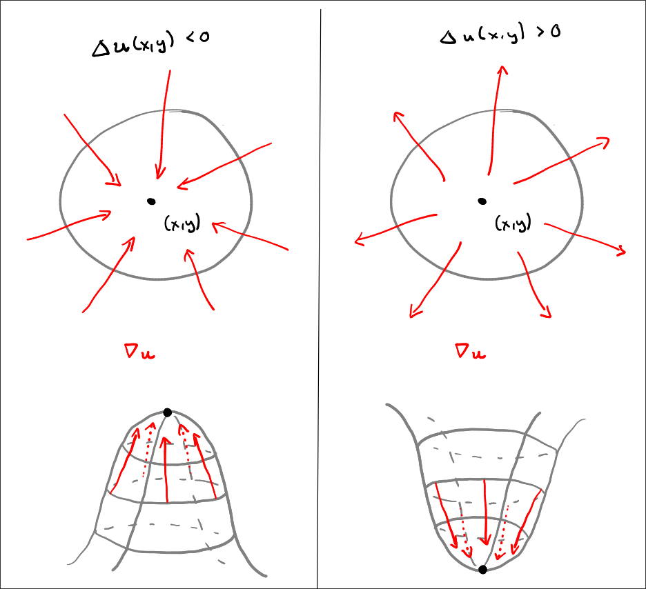
The influx in the above picture is represented by the laplacian \(\Delta u\). The gray space around the point \((x,y)\) would then be the other values which \(u\) takes on in a neighborhood around \((x,y)\).
How can we find \(u\) given the above poisson equation?
We will calculate the solution approximately on a grid